I will start with monodromies in the context of analytic continuation and linear differential equations, since that is where I encountered them first. Here are the current prerequistes for this article: complex numbers, Taylor series.
The basic problem goes back to the square root, when extended to the complex numbers. The school rules, such as \( (xy)^a = x^a y^a \), no longer work, as exemplified by $$-1 = \mathrm{i}\cdot\mathrm{i} = \sqrt{-1}\sqrt{-1} \overset{?}{=} \sqrt{1} = 1.$$ This happens, because of the root ambiguity, but could be blamed on poor notation and intuition inherited from (positive) real numbers. For \(r = \sqrt{w}\) means only that \(r\) satisfies \(r^2 = w\), and in that sense we do have \(\mathrm{i}^2=\sqrt{1}\), because \((\mathrm{i}^2)^2 = 1\). It is only when we call \(r\) the number that satisfies \(r^2=w\) that problems begin. Keeping track of all the roots consistently is thus the first priority.
In the general, complex case we go back to the equality \(\exp(\alpha)\exp(\beta)=\exp(\alpha+\beta)\), and recall that \(\exp\) is periodic. So that although \((e^{\alpha})^n = e^{n\alpha}\) gives an immediate root formula \(\sqrt[n\,]{e^{\beta}} = e^{\beta/n}\), we could just as well take \((e^{\alpha})^n = e^{n\alpha+2\pi k\mathrm{i}}\), \(k\in\mathbb{Z}\), giving a whole family of roots \(e^{\beta/n}e^{2\pi\mathrm{i}k/n}\).
Why do we care about the exponents? Firstly, because this is a straightforward way of defining arbitrary powers via \(z^a := \exp(a\ln(z))\), and we know everything about the exponential functions, including how many different solutions (roots) to expect1.1. According to the previous formula, there are only \(n\) essentially distinct values of \(k\) in the above formulae, e.g. \(\{0, 1,\ldots, n-1\}\), that give distinct complex roots.
Rephrasing the example with \(\exp\), we have \( (e^{\pi\mathrm{i}})^{1/2}(e^{\mathrm{i}\pi})^{1/2} = (e^{2\pi\mathrm{i}})^{1/2} = e^{\pi\mathrm{i}} = -1\), and all seems well. Except that, by periodicity, \(e^{2\pi\mathrm{i}} = e^0\), and clearly everyone must agree that \((e^0)^{1/2} = e^{0/2} = e^0 = 1\), so we're back where we started. If only there were some way to distinguish \(1=e^0\) from \(1=e^{2\pi\mathrm{i}}\)…
The second reason is that using functions shifts the focus from numeric (arithmetic) to analytic properties. We are not so much interested in how to compute the value of square root accurately (continued fractions of course!), but rather how the value changes as the argument moves around the complex plane. The representation \(z=\rho\,e^{\mathrm{i}\varphi}\), makes it painfully clear, that the modulus \(\rho\) plays little role, since it is non-negative; it's the argument \(\varphi\), whose loops give us the headache1.15.
On the one hand, the interval of \([0, 2\pi)\) is enough for \(\varphi\) to parametrize all the numbers, on the other, it makes intuitive sense to describe several revolutions around the origin, and use numbers such as \(4\pi\) or \(40\pi\) to quantify how the path winds. The paths \([0,2\pi) \ni \varphi\mapsto e^{\mathrm{i}\varphi}\) and \([0,10\pi) \ni \varphi\mapsto e^{\mathrm{i}\varphi}\) are different as functions, even though they are projected onto the same unit circle. (This hints at the fundamental group, which will come into play later.) And perhaps the roots “feel” the position on the full path (as given by the argument \(\varphi\)), not just the final value of \(z=e^{\mathrm{i}\varphi}\). So, let's look at the root, when followed along two different (half) loops.
Several choices have to be explained here. Why are both the roots initially \(1\) (\(\sqrt{w}\) could be \(-1\))? Because we are now paying attention to continuity — we wish for everything to lie close together initially, so if the arguments start at the same point, so should the roots. Secondly, why do the roots follow their arguments? Because once we decide they are close (start near \(1\) not \(-1\)), there is no other choice: say the root is \(1+\epsilon + \mathrm{i}\eta\), then its square (neglecting terms quadratic in \(\epsilon\) and \(\eta\)) must be \(1 + 2 \epsilon + 2\mathrm{i}\eta\), so the signs of the imaginary parts of \(u\) and \(\sqrt{u}\) are the same, as dictated by \(\eta\)1.75; and the respective roots must fall on either side of the real axis. Then the inevitable happens, when both numbers reach the negative semiaxis, and the imaginary parts no longer distinguish between them. And yes, we have long left the region of convergence of the Taylor series (going in opposite directions to make it even worse), so no wonder things break down. Let's try following just one path for as long as possible (for clarity the circles will be displaced slightly).
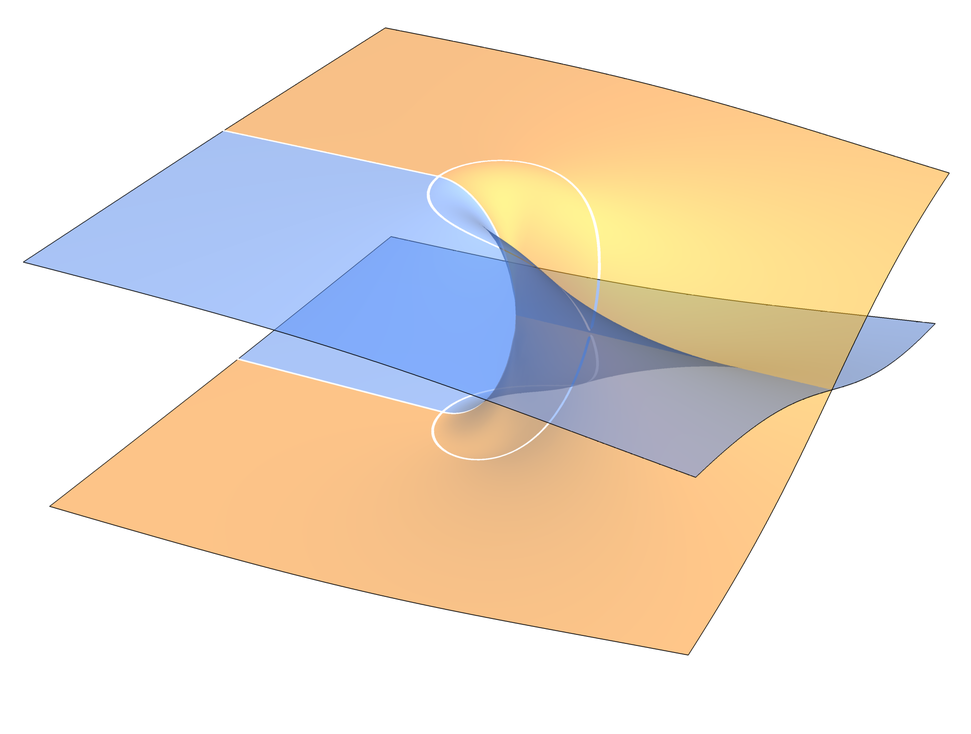
Right at the outset it has to be noted, that there is more than one way of doing this. I chose to follow the previous example and the surface image at the top: there is a transition at \(-1\) which the colours depict. This is not immediately obvious, because we can just accept that \(\sqrt{-1} = +\mathrm{i}\); but as the first full circle is complete, \(u\) should not be “the same” \(1\), because now the root has changed to \(\sqrt{u}=-1\). We solve this by claiming that now we are in the blue territory, as if \(u={\color{darkorange}1}\) and \(u={\color{blue}1}\) were distinct numbers. One could keep it orange until \(1\) is reached again, and make the transition there, but the point is that this transition must happen eventually.
The new territories should still correspond to our intuitions of (sets of) complex numbers, so we continue along the blue path, insisting that it should cover the whole angle of \(2\pi\) over which the argument varies. We passed to blue at \(-1\), and as we continue circling to it, nothing bad happens with the root: it circles from \(+\mathrm{i}\) to \(-\mathrm{i}\). At that point, we must go back to the orange territory. Thankfully we can: there's just an angle of \(\pi\) to cover, because the beginning of the path only made half a circle from \(0\) to \(-1\). With this final arc, we land back at \(u = {\color{darkorange}1}\), precisely in time when \(\sqrt{u}\) reaches \(1\) too.
And this is the solution: to consider \(u\) as living on two copies of the complex plane, such that the values of the square root each have their corresponding arguments. By demanding that the sheets are connected, so that the loop around \(0\) is consistent, we construct and visualize an abstract surface: the Riemann surface of \(\sqrt{z}\), as shown in our first attempt above.
All we had to do was give the path width by considering numbers of moduli other than exactly \(1\), which turns the circles into circular strips (or rings). Nothing essentially new happened here, the square root just lies on a circle of a different radius, and for positive radii we have a one-to-one correspondence. So both planes (for \(u\) and \(\sqrt{u}\)) should be fully covered, except that the above problem persists for all of them at the real negative semi-axis, i.e. when the loop is closed. Se we cut the complex plane there (leaving \(u=0\) out for now), create two coloured copies, and try to glue them back together like this:
And don't worry about the self-intersection — we will get rid of it later — it is an artifact of the construction in three dimensions. A useful byproduct of the intersection, however, is that it highlights the required cuts (more on that below), and shows which numbers to identify (\({\color{darkorange} 1}\) and \({\color{blue} 1}\)). In the end we will want the result of some calculation to be a single, “ordinary” complex number, so the surfaces will have to be squashed vertically, but before that, we look at them from above, and they need to align.
Once we distinguish between the sheets, things work wonderfully: $$ {\color{darkorange}-1} = \sqrt{\color{darkorange}-1}\sqrt{\color{darkorange}-1} = \sqrt{({\color{darkorange}-1})({\color{darkorange}-1})} = \sqrt{\color{blue}1} = {\color{darkorange}-1}, $$ whereas \(\sqrt{\color{darkorange}1}={\color{darkorange} 1}\), and there is no confusion, because each \(1\) gets its own (arithmetic) root. We can also clearly distinguish between \({\color{darkorange} \mathrm{i}}=\sqrt{\color{darkorange}-1}\) and \({\color{blue} -\mathrm{i}}=\sqrt{\color{blue}-1}\), for which, thankfully, \({\color{darkorange} \mathrm{i}}({\color{blue} -\mathrm{i}}) = {\color{darkorange} 1}\).
If a civilization lost the ability to print or see colour, all of the above formulae would still make sense, with the tiny modification that \(\sqrt{}\) be read as “some root of”; \(-\mathrm{i}\) is some root of \(-1\) after all. They (and present-day formalists) would still insist on introducing a rigorous notation, not to run afoul of arithmetic1.2 (or even just intransitivity of the relation “equal to some”). They could consider orange and blue to correspond to two components of a single vector like so: $$ {\color{darkorange} 1} = \begin{bmatrix} 1\\ +1 \end{bmatrix}, \quad {\color{blue}1} = \begin{bmatrix} 1\\ -1 \end{bmatrix},$$ with the second component encoding the expected root sign. And indeed any complex number, could be denoted by a pair, \((u,z)\), motivated by the definig equation \(u = z^2\). Then the number \(x=(4,-2)\), which would ordinarily be just \(4\), would have a unique square root of \(-2\) or rather \(\sqrt{x}=(-2,\mathrm{i}\sqrt{2})\). And although we now need two coordinates instead of one to keep track, we are always restricted to the surface of \(u = z^2\), so the complex dimension stays at \(1\) — the first number almost gives us the full information, while the second only encodes the sign.
I don't want to get into that too deeply here, because the next section will introduce a different representation still, one more in keeping with \(z\) being a single complex number. However, one important observation follow immediately from trying to make the notation rigorous: it breaks down on repeated application of the root. Because why couldn't we take \(\sqrt{x}=(-2,-\mathrm{i})\) in the above? The surface restriction is satisfied, and the first component, \(-2\) agrees with the original number's second component, i.e., \(\sqrt{(a,b)}=(b,\ldots)\). But of course, the dots are unspecified, for there is no third component to help. Simply put, we can have both \(u\) and \(z=\sqrt{u}\), but when you additionally ask for \(\sqrt{z}\) that means you really wanted the Riemann surface of \(\sqrt[4\,]{u}\) all along! No problem, it too can be constructed, but it's just not included by default in the construction for \(\sqrt{u}\).
Now that we have some understanding of the problems with complex cuts for the sequre root, and nice geometric intuitions to deal with them, we can look at \(\sqrt{z}\) as a complex function of \(z\), and its analytic properties. Specifically, the connection between its singularities and simple differential equations will lead directly to a practical understanding of what monodromy is.
So far we have mostly ignored what happens at \(z=0\), but in a way it is the most problematic point of all, because the function is not differentiable there, and the singularity is not even a pole, but an algebraic one. This fact was almost irrelevant before, and in fact \(0\) was the only number for which there was no problem of choosing the root value. At the same time, the problematic loops were precisely those around zero. There are many ways of arriving at the connection, one of which is through analytic continuation and differential equations.
What makes it the ideal simplest example, is that we can immediately obtain the relevant equation, which has only a pole: $$ \frac{\text{d}\sqrt{z}}{\text{d}z} = \frac{1}{2\sqrt{z}} \quad\Longrightarrow\quad f'(z) = \frac{1}{2z}f(z). \tag{E}$$ The smallest class of equations, which will dominate this article, will thus be linear differential equations with rational coefficients. And the root demonstrates, the solutions of even the simplest such equations are not rational themselves (not even algebraic in general, as we shall see). Rationality itself is brought to the fore for two reasons. First, rational functions form a field, \(\mathbb{C}(z)\), which is the basic structure supporting standard arithmetic: we want to multiply and divide our functions, just like (complex) numbers2.05. Second, although the equation could be rewritten as \(2zf'-f=0\), making it polynomial, solving it specifically for the derivative is what makes analytic continuation “easy”. Specifically, it immediately gives all derivatives by iteration: $$ \begin{aligned} f'' &= \left(\frac{1}{2z}f\right)' = -\frac{1}{2z^2}f + \frac{1}{2z}f' = -\frac{1}{4z^2}f,\\ f''' &= \left(-\frac{1}{4z^2}f\right)'\ = \frac{3}{8z^3}f,\quad\text{etc.} \end{aligned} $$
Thus, at any point other than \(z=0\), when given the initial value, we can obtain the whole Taylor series. It is an important result, that the series is always convergent, and I direct everyone to the classical textbook of Watson and Whittaker for details2.1. In theory, one can take another point, \(z_2\), inside the series' convergence region, calculate \(f(z_2)\) by summation, and then use that together with equation \((\mathrm{E})\) again to construct a new series, check its radius of convergence and so on. This way, the complex plane could be traversed, so long as we avoid the point \(z=0\).
You know where this is going — we will continue the series along the unit circle starting and ending at \(z=1\). At every step we will have a correct solution to \((\mathrm{E})\), each slightly different from the previous one, but at the same time continuos (analytic even), so that as the argument of \(z\) increases from \(0\) to \(2\pi\), the argument of \(f(z)=\sqrt{z}\) will increase from \(0\) to just \(\pi\). By the time the loop is closed, the value of \(f\) will thus necessarily be \(-1\) instead of \(1\). (The problematic cut-line will now be the real positive semi-axis, this choice is as widely used, so it's best to get used to both early.)
Right away it should be stressed that it is an abuse of notation, to just use the single letter \(f\) to denote the initial solution, its series, and all the subsequent series. These are all different. So we should have said, that the initial solution \(f_1\), such that \(f_1(1)=1\) gives rise to series \(S_1\), convergent in a circle of radius \(1\) around \(z_1=1\). It gives rise to the series \(S_2\) at another point, say \(z_2=(1+\mathrm{i})/\sqrt{2}\), and we wish its limit, \(f_2(z)\), to agree with \(f_1\) specifically at (and around) \(z_2\). We then move to \(z_3=\mathrm{i}\), and repeat. When finally \(z_8 = (1-\mathrm{i})/\sqrt{2}\) is reached, the resulting function \(f_n(z)\) is still a solution, but does it agree with \(f_1(z)\)? No, but it's nothing scary just \(-f_1(z)\). If we replaced \(z_i\) with a continuously moving point \(u\), it would like something like this:
This is where the linear character of the equation is essential, because the solutions form a vector space. It's one-dimensional, and using that language might seem too much right now, but it will soon become central. For now, we can focus on the continuation, while keeping in mind that all solutions of \((\mathrm{E})\) are of the form \(c \sqrt{z}\). This makes \(f_1(z)\) the fundamental solution, and all others are just some multiples. Crucially, the continuation process changed the solution with \(c=1\) to a solution with \(c=-1\). And indeed for an general solution \(g(z) = c\sqrt{z}\), its continuation leads to \(-g(z)\). This is enough to finally obtain our first group, because all we need now is analyze the repetition of the process.
There is essentially one interesting loop around zero, so let's denote it by \(\gamma\) and define $$ \mathsf{Cont}_{\gamma}(g) := \left| \begin{matrix} \text{the result of analytic} \\ \text{continuation of $g$ along $\gamma$} \end{matrix}\right| = -g.$$ If the loop is followed twice, like for the sheets previously, we could denote the loop by \(2\gamma\), or just write $$\mathsf{Cont_{2\gamma}} g = \mathsf{Cont}_{\gamma}\mathsf{Cont}_{\gamma} g = -(-g) = g.$$ As the root changes the sign back and forth, the only available operations are multiplication by \(-1\) or \(1\), so the group is simply \(\mathbb{Z}_2\) realized as \(\{1,-1\}\) with multiplication. This is the monodromy group for equation \((\mathrm{E})\).
In natural language, we could say that the solution (square root) generates a cut; passing through the cut requires the muliplication by \(-1\). The group shows all possible multiplications, arising when you travel around arbitrary paths. And they have to be closed, because comparing two functions should happen at the same point. They only differ by \((-1)^n\), where \(n\) is the number of revolutions around zero.
To more fully appreciate the group structure, we need higher order equations, which will bring the underlying vector space to the fore. So let's consider the following $$ f''(z) + \frac{1}{6z}f'(z) - \frac{1}{6z^2}f(z) = 0,$$ which, again, has a singularity at zero, and two algebraic solutions: $$ f_1(z) = \sqrt{z},\quad f_2(z) = z^{1/3},$$ so that any solution can be written as \( f = c_1 f_1 + c_2 f_2\), with complex constants \(c_i\). The iterative proces, to obtain a series solution term by term, works again, although this time one has to start with two initial conditions: the value of the function as well as the first derivative — the equation then gives the second and higher derivativs.
The vector space is thus two-dimensional, and so any solution can be given simply as \((c_1,c_2)\), with the understaing that the basis vectors are \(f_1\) and \(f_2\). The usual linear operations on the vector space represent the natural properties of the equation. E.g. the sum of two vectors \((c_1,c_2)+ (d_1,d_2) = (c_1+d_1,c_2+d_2)\) means that if \(f\) and \(g\) are solutions, so is their sum \(f+g\). We can also multiply a solution by a constant, but with the vector we can do more (or rather, we can notice more): multiply by a matrix, which mixes the components: $$ (c_1, c_2) \begin{pmatrix} m_{11} & m_{12} \\ m_{21} & m_{22} \end{pmatrix} = (m_{11} c_1 + m_{21}c_2, m_{12}c_1 + m_{22}c_2).$$ Although it is not immediately obvious how to interpret this (perhaps a change of basis), and why it is right-multiplication (see below), this operation is just what we need for monodromy.
For consider what happens when we complete the usual loops around zero. We already know everything about the square root: it gains factors of \(-1\). What of the cubic root? Likewise it will require to include the possible roots of \(x^3=1\). Let's define the primitive root to be \(\omega := e^{2\pi\mathrm{i}/3} = \frac12(-1+\sqrt{3}\mathrm{i})\). It's called primitive because all three can be written as \(\{\omega,\,\omega^2,\,\omega^3=1\}\). And by considering the parametrization of the loop by \(e^{\mathrm{i}\varphi}\), whose root is \(e^{\mathrm{i}\varphi/3}\), we come to the analogous result: $$ \mathsf{Cont}_{\gamma}z^{1/3} = \omega z^{1/3},$$ so that double continuation will produce the factor of \(\omega^2\); and the triple loop will bring us back to \(\omega^3 z^{1/3}=z^{1/3}\), after which he original function is restored — the Riemann surface has three sheets.
We can write this all together, rewriting \(c_1\sqrt{z}+c_2 \sqrt z^{1/3} \rightarrow -c_1 \sqrt{z} + c_2 \omega z^{1/3}\) in its vector form: $$ \mathsf{Cont}_{\gamma}(c_1,c_2) = (-c_1, \omega c_2) = (c_1, c_2) \begin{pmatrix} -1 & 0 \\ 0 & \omega \end{pmatrix} =: (c_1, c_2)M.$$ This \(M\) is the monodromy matrix for our equation around \(z=0\), it tells us what happens to the basis solutions, \(\sqrt{z}\) and \(z^{1/3}\), and by extension any solutions, after continuation. What is the full group, though? Thanks to the multiplicative properties of the equation, the group is realized as some matrix group, and since there are no other (continuation) operations, we can just iterate it to get $$ \begin{aligned} M_1 &= \begin{pmatrix} -1 & 0 \\ 0 & \omega \end{pmatrix}, && M_2 = M_1 M_1 = \begin{pmatrix} 1 & 0 \\ 0 & \omega^2 \end{pmatrix}, \\ M_3 = M_2 M_1 &= \begin{pmatrix} -1 & 0 \\ 0 & 1 \end{pmatrix}, && M_4 = M_3 M_1 = \begin{pmatrix} 1 & 0 \\ 0 & \omega \end{pmatrix},\\ M_5 = M_4 M_1 &= \begin{pmatrix} -1 & 0 \\ 0 & \omega^2 \end{pmatrix}, && M_6 = M_5 M_1 = \begin{pmatrix} 1 & 0 \\ 0 & 1 \end{pmatrix}, \end{aligned} $$ ending with the identity element. Diagonal matrices commute, so we get the cyclic group \(\mathbb{Z}_6\).
We now have essentially all notational tools, to deal with monodromies: we will consider them as some matrix groups, which describe what happens to the solutions of linear differential equations, as closed loops are taken around singularities. There is still one step to take, to fully work with matrices, and that is to rewrite the differential equation as a system. This will get rid of the row vectors \(c_1,c_2\) which lie somewhere between scalar and system notations.
Let's use the unkwnon function as the first component, \(h_1 = f(z)\) and the derivative as another component by taking \(h_2 = z f'(z)\). The equation then becomes $$ \frac{\text{d}}{\text{d}z} \begin{bmatrix} h_1\\ h_2\end{bmatrix} = \frac{1}{z}\begin{bmatrix} 0 & 1 \\ -\frac{1}{6} & \frac{5}{6}\end{bmatrix} \begin{bmatrix} h_1\\ h_2\end{bmatrix}, $$ with the singularity neatly brought to the front. The difference between this and the previous representation is that now we are still dealing with functions. From the definitions of \(h_i\) we get $$ f_1(z) = \sqrt{z} \longleftrightarrow H_1(z) = \begin{bmatrix} \sqrt{z} \\ \frac12 \sqrt{z} \end{bmatrix},\quad f_2(z) = z^{1/3} \longleftrightarrow H_2(z) = \begin{bmatrix} z^{1/3} \\ \frac13 z^{1/3} \end{bmatrix}.$$ These can be gathered in what is called the fundamental matrix, as columns: $$ F(z) = \begin{bmatrix} \sqrt{z} & z^{1/3} \\ \frac12 \sqrt{z} & \frac13 z^{1/3}\end{bmatrix},$$ which satisfies the same equation, i.e., $$ F'(z) = A(z)F(z), \qquad A(z) = \frac{1}{z}\begin{bmatrix} 0 & 1 \\ -\frac{1}{6} & \frac{5}{6}\end{bmatrix}.$$
The fundamental matrix must contain linearly independent columns (solutions), so that any other solution can be obtained from it. Note, that this is the case at (and around) \(z=1\), but not at \(z=0\), where the marix is not differentiable (we will come back to this point). Both the previous solutions are thus expressible, e.g., \(H_1 = F\, {1 \brack 0}\). The equation also makes it clear that right-multiplication by any \(2\times2\) constant matrix is allowed, i.e., \(F\, Q\) will always be a solution, and if \(\det{Q}\neq 0\) it will be another fundamental matrix.
Quite naturally we have $$ \mathsf{Cont}_{\gamma} F =: F M,$$ and the matrix is exactly the same as before. We can now clearly see what happens when the basis of solutions is changed to, say, \(\sqrt{z}\pm z^{1/3}\). This corresponds to taking a new fundamental matix $$ G = F\, Q, \quad Q = \begin{bmatrix} 1 & 1 \\ 1 & -1 \end{bmatrix},$$ and obtaining its continuation as $$ \mathsf{Cont}_{\gamma}G = \mathsf{Cont}_{\gamma}F Q = F M Q = G Q^{-1}M Q = : G \widetilde{M}.$$ Just an equivalnce transform between \(M\) and \(\widetilde{M}\), so everything is under control. We just have to keep in mind that the particular representation of the monodromy will depend on the choice of basis3.1.


Sed ne soli mihi hodie didicerim, communicabo tecum quae occurrunt mihi egregie dicta circa eundem fere sensum tria, ex quibus unum haec epistula in debitum solvet, duo in antecessum accipe. Democritus ait, 'unus mihi pro populo est, et populus pro uno'.
Bene et ille, quisquis fuit - ambigitur enim de auctore -, cum quaereretur ab illo quo tanta diligentia artis spectaret ad paucissimos perventurae, 'satis sunt' inquit 'mihi pauci, satis est unus, satis est nullus'. Egregie hoc tertium Epicurus, cum uni ex consortibus studiorum suorum scriberet: 'haec' inquit 'ego non multis, sed tibi; satis enim magnum alter alteri theatrum sumus'.
Ista, mi Lucili, condenda in animum sunt, ut contemnas voluptatem ex plurium assensione venientem. Multi te laudant: ecquid habes cur placeas tibi, si is es quem intellegant multi ? introrsus bona tua spectent. Vale.
| 1.1 | The appearance of the logarithm might seem circular — isn't it defined as the inverse of \(\exp\) and multivalued on top of that? — but it captures precisely the ambiguity of \(\beta\) when representing \(x\) as \(e^{\beta},\) so that we can deal with it explicitly. If \(a\) is an integer, the ambiguitiy is irrelevant, otherwise we know exactly what choices are left. The usual perverse example is \(\mathrm{i}^{\mathrm{i}}\), for which \(\ln(\mathrm{i}) = (2k+\frac{1}{2})\pi\mathrm{i}\), so in the end we get \( e^{-\pi(4k+1)/2}\) — infinitely many distinct real values. |
| 1.15 | Those familiar with a littel bit of differential geometry will protest, that \(\rho\) is just as guilty, because the change of coordinates from \(z=a+\mathrm{i}b\) to \(z=\rho e^{\mathrm{i}\varphi}\) is singular at \(\rho=0\). But that is begging the question, as we are trying to get to the bottom of what precisely goes wrong. It is no coincidence, that we have chosen the loops to go around zero specifically, but at the same time, there is no need for \(\rho\) to apprach zero for the problems to appear. Still, as is usually the case, it is not one or the other — the different perspectives are complimentary and entangled, such is the beauty of maths. |
| 1.75 | This foreshadows the analytic properties. We expect the root, as a function, to behave nicely (analytically) around \(1\). Its Taylor expansion gives \(\sqrt{1+z}\approx 1+\frac{1}{2}z\), so that for \(z\) close to the real axis \(\mathrm{Im}(\sqrt{u}) = \frac12\mathrm{Im}(u) >0\), while \(\mathrm{Im}(\sqrt{w})< 0\), |
| 1.2 | For consider the equality \(\sqrt{\color{blue}1} = {\color{orange}-1} = {\color{orange}-}\sqrt{\color{orange}1}\), which becomes \(\sqrt{1} = -\sqrt{1}\) when projected to black and white, and just \(1=-1\) on division. Or \(\sqrt{\color{blue}1}+\sqrt{\color{orange}1}=0\), leading to \(2\sqrt{1}=0\). Except of course, those simplifications are unjustified, for we can at best write \(\sqrt{1}/\sqrt{1}=1\) (some root of one divided by some root of one is minus one) in the former, and \(\sqrt{1}+\sqrt{1}=0\) (some root of one plus some root of one is zero) in the latter. It's the qualifier some doing all the heavy lifting (and confusing). |
| 2.05 | There is an even deeper reason here, when one starts asking about solvability of differential equations. To meaningfully ask, whether an equation can be solved, one has to specify the allowed methods or, in this case, classes of functions. Rational functions are one such closed class, because they form a differential field, where derivatives are added to arithmetic. They are, as we have seen, insufficient as the solution space, and the investigation of the reasons gives rise to the differential Galois theory. Just like with its ordinar version, which explains why there are no general formulae for the roots of a quintic (with surds), and why the circle can't be squred (with only the ruler and compass being allowed), its differential variant introduces extensions of rational or meromorphic functions, and gives criteria of solvability. |
| 2.1 | E. T. Whittaker and G. N. Watson, A course of Modern Analysis. I cannot recommend this book highly enough. Though it's over a century old, the level of detail and clarity is unsurpassed. If you want to learn how to actually solve linear differential equations this is the textbook. Of course it comprises many more branches of analysis too, most notably the elliptic functions of Weierstrass and Jacobi. It's a great remedy to the modern Bourbakian gobbledygook. |
| 3.1 | Alternatively, one defines holonomy matrix \(K\) (and then the holonomy group) to be the matrix inserted on the left: $$ \mathsf{Cont}_{\gamma} F =: K F.$$ This makes it basis independent, as all the right factors will cancel. It's a matter of convenience which to use. |